Components of Reproducible-ML

In this section, we will show how the components of a Machine Learning (ML) pipeline are embedded in Reproducible-ML and highlight their relationship towards each other. Similar to the overview in The Concept of Reproducible-ML section we start with basic data pre-processing and go through all steps of the pipeline until we reach the output.

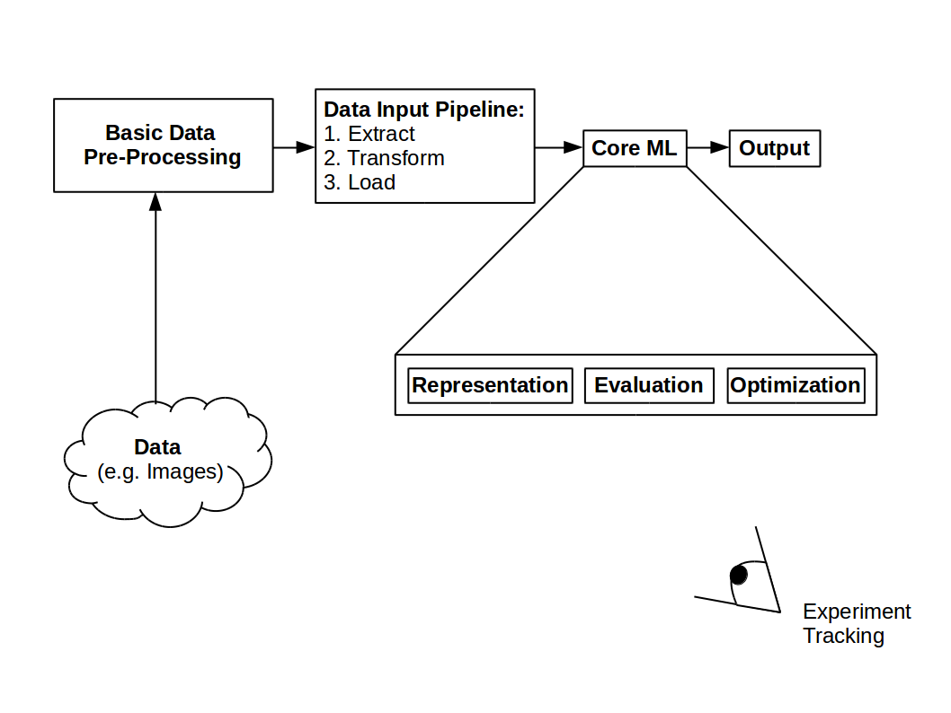
Machine learning pipeline overview

Basic Data Pre-Processing

In Reproducible-ML the basic pre-processing is implemented with the help of two steps. The Handler module which takes as input the raw data and outputs TensorFlow features and the conversion which takes TensorFlow features and outputs TensorFlow record files. We call this process serialization.

Storing the data in binary files (i.e. .tfrecords) brings several advantages. One of them is the image and its annotations are stored in a single block of memory compared to storing each image and its annotations separately. Overall, using binary files makes the reading of data much more efficient.

Detailed view of Basic Data Pre-Processing

Handlers

Within the handler module, things like image scaling, slicing, reshaping etc. are done. Each handler inherits from a base class called FeatureHandler. Have a look at Handler package for more information concerning the base class. Lets consider an easy example, we have as raw input images of size [91,91] and we want to rescale them to [128,128] and return the images in TensorFlow bytes feature. The following code snipped shows such a Handler:

class TestHandler(FeatureHandler):
    """Handler to rescale images from [91,91] to [128,128]

    Loads images using an returns byte features.

    Attributes:
        img_folder (str): Path to folder containing the images.
        img_shape (list of int): Desired shape for the images.
        img_dtype (str): Desired data type for the images.
    """
    def __init__(self, img_folder, img_shape, img_dtype):
        super(TestHandler, self).__init__(delegate_to=None, shape=[])
        self.img_folder = img_folder
        self.img_shape = img_shape
        self.img_dtype = getattr(np, img_dtype)

    def handle(self, row, key):
        img = np.load(img_path)

        if self.img_shape != list(img.shape):
            img = scipy.misc.imresize(img, self.img_shape)

        img_feature = {}
        img_feature[key] = utils.bytes_feature(img.tostring())

        return img_feature

The image features are grouped as python dictionaries and for this simple case the key could simply be “image”. The function which transforms the rescaled images to byte features is implemented in the Utils module. Have a look at Utils package for other possible features.

Conversion

The Conversion is simply done by binarizing the TensorFlow features and save them as .tfrecods. A template for the conversion step called write_records is presented here:

def write_records(record_dir,
              record_pattern,
              keys_to_handlers,
              samples_per_record,
              split_to_size,
              rows_gen):


    record_pattern = mkdir_and_join(record_dir, record_pattern)

    for split in ["train", "eval", "test"]:

        rgen = rows_gen(split)

        n_records, n_samples_left = div_mod(split_to_size[split],
            samples_per_record)

        for idx in range(n_records):

            writer, record_path = get_writer(record_pattern, split, idx)
            write_samples(samples_per_record, rgen, keys_to_handlers, writer)

        if n_samples_left > 0:

            writer, _ = get_writer(record_pattern, split, n_records)
            write_samples(n_samples_left, rgen, keys_to_handlers, writer)

For more information concerning the functions div_mod, get_writer and write_samples please have a look at datasets.serialize module, however the names should be self-explanatory.

Serialization

To finalize the basic data pre-processing we bring together the handler and the conversion what we then call serialization. We need to choose which kind of handler we are going to use e.g. TestHandler and what kind of serialization will take place i.e. serialization from a NPZ file:

def config(npz_file):

    img_shape = [128, 128]
    img_dtype = "uint8"

    keys_to_descriptions = {"image": "Digit Image"}
    keys_to_handlers = {"image": TestHandler()}


def serialize(npz_file, key):

    serialize_npz(npz_file=npz_file, key=key)

You can test the basic pre-processing step by producing .tfrecord files from the MNIST data set following the first two steps of Experiments on MNIST Database.

Data Input Pipeline

Since Reproducible-ML uses the TensorFlow Estimator Module [8], the first two phases Extract and Transfrom are captured in an input function. A simplified input function could therefore be:

def input_fn():

        def fn():

            dataset = dataset_from_records("/path/to/dataset/train-*.tfrecord")
            dataset = tf.data.TFRecordDataset(tf.data.TFRecordDataset)
            dataset = dataset.map(map_func=map_fn())
            dataset = dataset.batch(batch_size)
            dataset = shuffle_repeat_prefetch(dataset)

        return dataset

    return fn

The data is now ready for being loaded onto any accelerator device to execute the core ML.

The Core of Machine Learning

This part is explained by means of a Generative Adversarial Network (GAN) [13]. GANs are ML algorithms consisting of two contesting neural networks, a Generator and a Discriminator/Critic. The Generator learns to generate samples while the Critic tries to distinguish between generated and real samples. For more information about GANs please refer to [13].

As introduced in The Concept of Reproducible-ML we follow the idea of [12], that a learning process consists of combinations of three components:

1. Representation: The Generator and the Critic network. Here a simplified example of a Generator network which takes in a noise vector and returns a generated 28x28 image:

def generator_fn(gan_type):

    def generator(noise):

        with tf.name_scope("critic") as scope:

            layer = layers.fully_connected(noise, 1024)
            layer = layers.fully_connected(layer, 7*7*256)
            layer = tf.reshape(layer, [-1, 7, 7, 256])
            layer = layers.conv2d_transpose(layer, 64, [4,4], stride=2) # 14x14
            layer = layers.conv2d_transpose(layer, 32, [4,4], stride=2) # 28x28
            layer = layers.conv2d(layer, 1, [4,4], stride=1,
                                  activation_fn=tf.tanh,
                                  normalizer_fn=None)

            return layer
    return generator

And an example of a Critic network which takes as input an image and returns a value based on which real and fake samples are be distinguished:

def critic_fn(gan_type):

    def critic(images):

        with tf.name_scope("critic") as scope:

            layer = layers.conv2d(images, 64, [4,4], stride=2) # 14x14
            layer = layers.conv2d(layer, 128, [4,4], stride=2) # 7x7
            layer = layers.conv2d(layer, 1, [4,4], stride=2) # 7x7

            return tf.reduce_mean(layer)

    return critic

2. Evaluation: As evaluation metric we use the Wasserstein-loss introduced in [7], in which an approximation of the earth mover’s distance is used.

3. Optimization: To find the best target representation i.e. the best Generator and the best Critic we use the RMSProp algorithm [9].

It is important to notice that since Reproducible-ML is based on the TensorFlow Estimator, changing 2. and/or 3. is very easy, therefore it makes Reproducible-ML flexible. At the same time, change either of them you do not need to dig deeply in the code, which makes it also very simple. Let`s have a look at a possible training process:

def main():

    config = tf.estimator.RunConfig(model_dir=model_dir)

    gan_estimator = tfgan.estimator.GANEstimator(
        generator_fn=generator_fn(gan_type),
        discriminator_fn=critic_fn(gan_type),
        generator_loss_fn=tfgan.losses.wasserstein_generator_loss,
        discriminator_loss_fn=tfgan.losses.wasserstein_discriminator_loss,
        generator_optimizer=tf.train.RMSPropOptimizer(gen_lr),
        discriminator_optimizer=tf.train.RMSPropOptimizer(crit_lr),
        config=config
    )
    gan_estimator.train(input_fn())

Have a look at [4] for different kinds of evaluation metrics and [5] for other optimization techniques.

The output of this training process are generated images. Have a look at some sample output Experiments, and then you can start with your own ML pipeline.

Experiment Tracking

As mentioned in The Concept of Reproducible-ML tracking of experiments is of great importance. To integrate this part into our framework as easy as possible, we use Sacred. Following the description of [14] the core abstraction is the Experiment class in combination with the configuration of an experiment. Let`s have a look at a simple example:

from sacred import Experiment

ex = Experiment()

@ex.config
def config():
    samples_per_record = 10
    compression = "GZIP"


@ex.automain
def main(samples_per_record, compression):
    print(samples_per_record)
    print(compression)

You can know either run the code using the default settings:

python -m test_sacred -m sacred

which leads to the following output:

WARNING - test_sacred - No observers have been added to this run
INFO - test_sacred - Running command 'main'
INFO - test_sacred - Started run with ID "32"
10
GZIP
INFO - test_sacred - Completed after 0:00:00

or run it from the command line:

python -m test_sacred with samples_per_record=20 compression="ZIP" -m sacred

leading to the following output:

WARNING - test_sacred - No observers have been added to this run
INFO - test_sacred - Running command 'main'
INFO - test_sacred - Started run with ID "33"
20
ZIP
INFO - test_sacred - Completed after 0:00:00

We can open SacredBoard via:

sacredboard -m sacred

The output displayed on SacredBoard for the second run will therefore look like this:

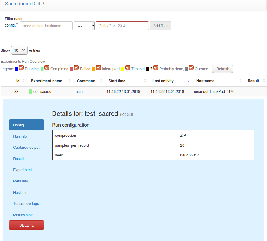
Print screen of ScaredBoard

There are also other nice and important features from Sacred which are used in Reproducible-ML. Please have a look at [2] for a complete documentation of Sacred.